Understanding the finite difference scheme (manual computations)

Lets do a good recap about a more specific problem I will focus to solve. The differential equation I want to solve is the following

\begin{align*} \frac{\partial^2 u }{\partial t^2} &= c^2 \frac{\partial^2 u}{\partial x^2} && \text{for } (x,t) \in (0,L) \times (0,T] \\ u(x,0) &= I(x) && \text{for } x \in (0,L) & \text{(Initial Position)} \\ \frac{\partial}{\partial t} u(x,0) &= 0 && \text{for } x \in (0,L) & \text{(Initial Velocity)}\\ u(0,t) &= 0 && \text{for } t \in (0,T] & \text{(Dirichlet Boundary Condition)}\\ u(L,t) &= 0 && \text{for } t \in (0,T] & \text{(Dirichlet Boundary Condition)} \end{align*}

For this particular problem, $c,I(x)$ must be prescribed to get an specific solution.

Given these conditions, we are going to discretize our domain i.e. we are generating a partition of the $(0,L) \times (0,T]$ domain as follows.

\begin{align*} x_i && \text{for } && i = 0, \dots ,N_x && \text{where } x_0 = 0 < x_1 < \dots < x_{N_x} = L \\ t_n && \text{for } && n = 0, \dots ,N_t && \text{where } t_0 = 0 < t_1 < \dots < t_{N_t} = T \end{align*}

The solution $u(x,t)$ is sought at the meshpoints. For notation, we will denote $u_i^n$ the approximation at the point $(x_i,t_n)$.

In this notation we assume a uniform partition, therefore $\Delta x = L/N_{x}$ and $\Delta t = T/N_t$

The partial differential equation

$$ \frac{\partial^2 u }{\partial t^2} = c^2 \frac{\partial^2 u}{\partial x^2} $$

Will be approximated using the following finite difference scheme

$$ \frac{u_i^{n+1} - 2u_{i}^n + u_i^{n-1}}{\Delta t^2} = c^2 \frac{u_{i+1}^{n} - 2u_{i}^n + u_{i-1}^{n}}{\Delta x^2} $$

If we define

\begin{align*} C = c \frac{\Delta t}{\Delta x} && \text{Famously known as the Courant Number} \end{align*}

That will lead us to the following recursion

$$ u_{i}^{n+1} = 2u_{i}^{n} - u_{i}^{n-1} + C^2 ( u_{i+1}^{n} - 2u_{i}^n + u_{i-1}^{n}) $$

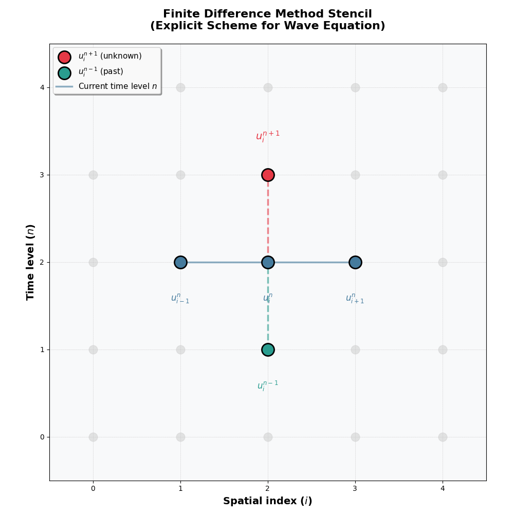
The recursion suggests that in order to find $u_{i}^{n+1}$ we will need to know $u_{i}^{n},u_{i}^{n-1},u_{i+1}^{n},u_{i-1}^{n}$, thats where the initial position, velocity and Dirichlet Boundary Conditions will help (but we will talk about that in more detail later). The technical word for that is an stencil.

This image illustrates the recursion process a.k.a the stencil.

.

Understanding how the initial velocity helps towards the solution approximation

Take the recursion previously provided for $n=0$, notice that it will produce the following equation.

$$ u_{i}^{1} = 2u_{i}^{0} - u_{i}^{-1} + C^2 ( u_{i+1}^{0} - 2u_{i}^0 + u_{i-1}^{0}) $$

Everything seems to be known or possible to be found, but, what is the meaning of $u_i^{-1}$ ? It might have different physical interpretations, but from a purely mathematical point of view we will use the initial velocity condition together with the centered finite difference method approximation to find $u_i^{-1}$.

With that being said, the initial velocity can be expressed in our finite mesh using the following approximation

$$ u_t(x_i,0) \approx \frac{u_i^1 - u_i^{-1}}{2 \Delta t} $$

Based on the initial velocity

$$ \frac{u_i^1 - u_i^{-1}}{2 \Delta t} = 0 $$

And

$$ u_i^1 = u_i^{-1} $$

Replacing it in the initial equation we will find that

$$ u_i^1 = u_i^0 + \frac{1}{2} C^2 (u_{i+1}^0 - 2u_{i}^0 +u_{i-1}^0) $$

Which will be used as we are applying the recursion $i=1,1,..,N_x-1$.

Applying the concepts to an actual problem.

Take the following partial differential equation

\begin{align*} \frac{\partial^2 u }{\partial t^2} &= c^2 \frac{\partial^2 u}{\partial x^2} && \text{for } (x,t) \in (0,L) \times (0,T] \\ u(x,0) &= A \sin( \left(\pi/L \right) x) && \text{for } x \in (0,L) & \text{(Initial Position)} \\ \frac{\partial}{\partial t} u(x,0) &= 0 && \text{for } x \in (0,L) & \text{(Initial Velocity)}\\ u(0,t) &= 0 && \text{for } t \in (0,T] & \text{(Dirichlet Boundary Condition)}\\ u(L,t) &= 0 && \text{for } t \in (0,T] & \text{(Dirichlet Boundary Condition)} \end{align*}

which has an analytical solution

$$ u_e(x,t) = A \sin( \left( \pi/L \right) x) \cos( \left( \pi/L \right) ct) $$

With $c=2,A=2,L=1,T=1$ and compute manually the expected results from partitioning the domain with $\Delta x = 1/4,\Delta t = 1/8$, we immediately see that the Courant number is $C=1$.

We start by applying the initial position condition $u(x,0) = 2 \sin(\pi x)$ and we find that

\begin{align*} u_0^0 &= 2 \sin(\pi*0) &= 0 \\ u_1^0 &= 2 \sin(\pi/4) &= \sqrt 2 \\ u_2^0 &= 2 \sin(\pi/2) &= 2 \\ u_3^0 &= 2 \sin(3 \pi/4) &= \sqrt 2 \\ u_4^0 &= 2 \sin(\pi) &= 0 \end{align*}

Lets use the initial velocity recursion we found previously, based on the specific problem we are solving that gives us

$$ u_i^1 = u_i^0 + \frac{1}{2} (u_{i+1}^0 - 2u_{i}^0 + u_{i-1}^0) $$

Based on that we conclude that

\begin{align*} u_1^1 &= 1 \\ u_2^1 &= \sqrt 2\\ u_3^1 &= 1 \\ \end{align*}

Given the Dirichlet Boundary conditions we are ready to apply the rest of the recursion, since $u_{i}^{n},u_{i}^{n-1},u_{i+1}^{n},u_{i-1}^{n}$ are known for $i=2,..,N_x -1$ and $t=2,..,N_t -1$

With this conceptual clarity lets implement an specific python class that solves this particular problem.

from typing import Tuple
import numpy as np
from numpy.typing import NDArray

"""
This is not a general PDE solver. It is a particular solver for the wave equation:
    u_{tt} = c^2 u_{xx}

with initial conditions:
    u(x,0) = A sin((pi/L)x)
    u_t(x,0) = 0

and boundary conditions:
    u(0,t) = 0
    u(L,t) = 0

We are solving this particular equation because it has an analytical solution:
    u(x,t) = A sin((pi/L)x)cos((pi/L)ct)

This allows us to compare our Finite Difference Method (FDM) solution to the analytical solution.

This implementation assumes the following parameter values:
    c = 2 (wave speed)
    A = 2 (amplitude)
    L = 1 (spatial domain length)
    T = 1 (time domain length)

Note: The reader is welcome to generalize this implementation to a more general wave equation 
FDM scheme or to include c, A, L, and T as general parameters if desired.
"""

class OneDimWaveFDM:

    _grid: Tuple[NDArray[np.float64], NDArray[np.float64]]
    _Nx: int
    _Nt: int
    _C: float  # Courant number (recursion constant): C = c*dt/dx
    _u: NDArray[np.float64]  # Solution array

    def __init__(self, Nx: int, Nt: int) -> None:
        self.Nx = Nx  # Uses setter
        self.Nt = Nt  # Uses setter
        self.create_raw_grid()
        self.compute_courant_number()
        self.initialize_solution()
        self.apply_initial_conditions()
    
    @property
    def grid(self) -> Tuple[NDArray[np.float64], NDArray[np.float64]]:
        """Get the grid."""
        return self._grid
    
    @grid.setter
    def grid(self, grid: Tuple[NDArray[np.float64], NDArray[np.float64]]) -> None:
        """Set the grid."""
        self._grid = grid
    
    @property
    def Nx(self) -> int:
        """Get the number of spatial grid points."""
        return self._Nx

    @Nx.setter
    def Nx(self, Nx: int) -> None:
        """Set the number of spatial grid points."""
        if Nx <= 0:
            raise ValueError("Nx must be positive")
        self._Nx = Nx

    @property
    def Nt(self) -> int:
        """Get the number of time steps."""
        return self._Nt
    
    @Nt.setter
    def Nt(self, Nt: int) -> None:
        """Set the number of time steps."""
        if Nt <= 0:
            raise ValueError("Nt must be positive")
        self._Nt = Nt


    @property
    def C(self) -> float:
        """Get the Courant number."""
        return self._C
    
    @C.setter
    def C(self, C: float) -> None:
        """Set the Courant number."""
        self._C = C

    @property
    def u(self) -> NDArray[np.float64]:
        """Get the solution array."""
        return self._u
    
    @u.setter
    def u(self, u: NDArray[np.float64]) -> None:
        """Set the solution array."""
        self._u = u

    def initialize_solution(self) -> None:
        self.u = np.zeros((self.Nx, self.Nt))
    
    def compute_courant_number(self) -> None:
        dx = 1 / (self.Nx - 1)  # Spatial step size
        dt = 1 / (self.Nt - 1)  # Temporal step size
        self.C = 2 * dt / dx
        
        # Check stability condition for explicit scheme
        if self.C > 1.0:
            recommended_Nt = int(np.ceil(2 * (self.Nx - 1))) + 1
            raise ValueError(
                f"Unstable Courant number: C = {self.C:.4f} > 1.0. "
                f"For stability with Nx={self.Nx}, need Nt >= {recommended_Nt}"
            )
    
    def create_raw_grid(self) -> None:
        """Create the spatial and temporal grid using meshgrid."""
        x = np.linspace(0, 1, self.Nx)  # Spatial points from 0 to L=1
        t = np.linspace(0, 1, self.Nt)  # Time points from 0 to T=1
        self.grid = np.meshgrid(x, t, indexing='ij')

    def apply_initial_conditions(self) -> None:
        self.apply_initial_displacement()
        self.apply_initial_velocity()   


    def apply_initial_displacement(self) -> None:
        X,_ = self.grid
        i = range(1,self.Nx-1)
        x = X[i,0]
        self.u[i,0] = 2*np.sin(np.pi*x)

    def apply_initial_velocity(self) -> None:        
        for i in range(1,self.Nx-1):
            self.u[i,1] = self.u[i,0] + 0.5*self.C**2 * (self.u[i+1,0] - 2*self.u[i,0] + self.u[i-1,0])


    def apply_boundary_conditions(self) -> None:
        self.u[0,:]=0
        self.u[-1,:]=0
    

    def solve(self)-> None:
        for n in range(1,self.Nt-1):
            for i in range(1,self.Nx-1):
                self.u[i,n+1] = -self.u[i,n-1] + 2*self.u[i,n] + self.C**2 * (self.u[i+1,n] - 2*self.u[i,n] + self.u[i-1,n])


def analytical_solution(x,t):
    """Analytical solution for comparison."""
    c = 2
    A = 2
    L = 1
    return A * np.sin((np.pi / L) * x) * np.cos((np.pi / L) * c * t)

Error Analysis

This is the plan for the error analysis.

• We will perform $m$ simulations
• The first simulation will be with a given $\Delta x_0,\Delta t_0$
• In each simulation $i=1,2,3,...$ we will decreased the size of $\Delta t_0$ by $\Delta t_i = 2^{-i} \Delta t_0$
• The value of the $u_{\text{approx}}(x_{N_x},t_{N_x})$ approximation will be compared to the analytical value $u_{\text{exact}}(x_{N_x},t_{N_x})$
• That will produce an array of errors $E_i$ which will be used with the $L^2$ norm to study the convergence error as $\Delta t$ decreases

import numpy as np
import matplotlib.pyplot as plt
import warnings
warnings.filterwarnings('ignore')


def analytical_solution(x,t):
    """Analytical solution for comparison."""
    c = 2
    A = 2
    L = 1
    return A * np.sin((np.pi / L) * x) * np.cos((np.pi / L) * c * t)

# --- Simulation Setup ---
m = 7 # Number of refinements
Nx0 = 10
Nt0 = 40 # Increased to ensure C is well below 1.0 throughout refinement

l2_errors = []
delta_t_array = []

for i in range(m):
    # Standard refinement: double the intervals, add 1 for the endpoint
    Nx = (Nx0 - 1) * 2**i + 1
    Nt = (Nt0 - 1) * 2**i + 1
    
    # Use your class
    simulator = OneDimWaveFDM(Nx, Nt)
    simulator.solve()
    
    X, T = simulator.grid
    dx = 1.0 / (Nx - 1)
    dt = 1.0 / (Nt - 1)
    
    # --- Error Analysis at Final Time ---
    u_approx_final = simulator.u[:, -1]
    u_exact_final = analytical_solution(X[:, -1], T[:, -1])

    error_final = u_exact_final - u_approx_final
    # Spatial L2 norm: sqrt( dx * sum(e^2) )
    l2_e = np.sqrt(dx * np.sum(error_final**2))
    
    l2_errors.append(l2_e)
    delta_t_array.append(dt)
    print(f"Level {i}: Nx={Nx}, Nt={Nt}, dt={dt:.5f}, L2_Error={l2_e:.2e}")

# Plot 1: Log-Log Error Convergence (separate figure)
fig1, ax1 = plt.subplots(figsize=(10, 6))
ax1.loglog(delta_t_array, l2_errors, 'o-', label='L2 Error', linewidth=2.5,
           markersize=8, color='#2E86AB')
# Reference line for O(dt^2)
# ax1.loglog(delta_t_array, [l2_errors[0]*(d/delta_t_array[0])**2 for d in delta_t_array], 
#            '--', color='gray', label='Theoretical $O(\Delta t^2)$')
ax1.set_xlabel('Time step size ($\Delta t$)', fontsize=12, fontweight='bold')
ax1.set_ylabel('L2 Error', fontsize=12, fontweight='bold')
ax1.set_title('Error Convergence: 1D Wave Equation FDM', fontsize=14, fontweight='bold', pad=15)
ax1.grid(True, which="both", alpha=0.3, linestyle='--', linewidth=0.7)
ax1.legend(loc='best', framealpha=0.9, fontsize=10, shadow=True)
ax1.set_facecolor('#F8F9FA')
fig1.patch.set_facecolor('white')
plt.tight_layout()
plt.show()

Level 0: Nx=10, Nt=40, dt=0.02564, L2_Error=4.47e-04
Level 1: Nx=19, Nt=79, dt=0.01282, L2_Error=2.79e-05
Level 2: Nx=37, Nt=157, dt=0.00641, L2_Error=1.74e-06
Level 3: Nx=73, Nt=313, dt=0.00321, L2_Error=1.09e-07
Level 4: Nx=145, Nt=625, dt=0.00160, L2_Error=6.80e-09
Level 5: Nx=289, Nt=1249, dt=0.00080, L2_Error=4.25e-10
Level 6: Nx=577, Nt=2497, dt=0.00040, L2_Error=2.66e-11